
By Peter Hecht, Ph. D., Vice President, Senior Investment Strategist at Evanston Capital Management
EXECUTIVE SUMMARY
• Markowitz’s “mean-variance” modern portfolio theory (“MV-MPT”) teaches us to evaluate investments, including hedge funds, in the context of the entire portfolio. Within MV-MPT, investors want to form portfolios with the highest Sharpe Ratio, i.e. maximize expected excess return for a given level of volatility (risk). New investments are judged based on their ability to increase the total portfolio’s Sharpe Ratio.
• Appraisal Ratio (“AR”), a risk-adjusted performance statistic, accounts for a new investment’s expected return, risk and diversification attributes in a manner consistent with MV-MPT. A higher AR translates to a higher total portfolio Sharpe Ratio.
• In order to calculate the AR, the key performance metric in MV-MPT, returns need to be beta-adjusted.
• Although AR is critical to investment evaluation in MV-MPT, it is not widely known or widely used; however, it is easily calculated using many common software programs.
• There are a number of misperceptions held with regard to portfolio performance evaluation, including too much focus on an individual investment’s Sharpe Ratio, expected return, and correlation properties. In contrast, there is too little focus on the importance of beta-adjusting returns and risk-adjusting alphas.
INTRODUCTION
Benchmarking hedge funds can be challenging, but as a former finance professor, I experience heartburn every time I hear the investment community criticize hedge funds for not keeping up with the S&P 500. It is the same type of heartburn I felt when investors thought hedge funds demonstrated skill when they outperformed the S&P 500 in 2008. Both comments reflect a fundamental misunderstanding on how to evaluate hedge funds……or any new investment.
Starting with Harry Markowitz in the 1950’s, “mean-variance” modern portfolio theory (“MV-MPT”) has taught us that investments need to be evaluated in the context of the investor’s entire portfolio – NOT in isolation. Specifically, investors want to know if having access to a new investment improves their entire portfolio’s expected return for a given level of total portfolio risk, i.e. improves the efficient frontier.
In practice, it is common for asset allocation specialists to discuss efficient frontiers with institutional investors. Separately, asset managers and other investment professionals report a full array of performance and risk statistics on various asset classes, strategies, and specific investment products. It is typically unclear how those performance and risk statistics relate to the investor’s ultimate goal of improving the efficient frontier. In fact, the long list of “jargon filled” statistics is often overwhelming and confusing.
If improving the efficient frontier is the ultimate goal, is it easy for the investor to simultaneously account for and evaluate an investment’s expected return, risk, and diversification attributes? Fortunately, the answer is yes [1]. The little known Appraisal Ratio (“AR”), an alpha consistency measure (defined as the ratio of an investment’s expected alpha to the expected volatility of its alpha), does just that. Within the set of new investments being considered, it can be shown that the investment with the highest AR improves the efficient frontier the most.
In order to calculate the AR (to be discussed later), an investment’s beta is necessary, as it is crucial to beta-adjust returns when evaluating performance – whether it be for a hedge fund or any investment product (please digest and refer to the opening paragraph). While they are all related, it is important to note that the AR is different than the widely used Sharpe Ratio or “plain vanilla” alpha measures.
But first, let’s head back to class and briefly review the core concepts of Markowitz’s Nobel Prize winning MV-MPT.
MARKOWITZ’S MODERN PORTFOLIO THEORY – A BRIEF REVIEW
In Markowitz’s classic MV-MPT, investors are assumed to have “mean-variance” preferences: for a given level of expected return, less variance[2] (or volatility) is preferred, or for a given level of variance, more expected return is preferred. This criterion defines the efficient frontier – the set of optimal portfolios to consider. When a risk-free asset (e.g. Treasury Bills or “T-bills”) and borrowing/lending are available, these preferences imply that investors want to form portfolios that maximize the Sharpe Ratio, which is defined as the total portfolio’s expected excess return (in excess of T-bills) divided by total portfolio volatility. This is why the Sharpe Ratio is one useful measure to consider at the total portfolio level[3].
In this unconstrained world, it can be shown that the efficient frontier, i.e. portfolios with the highest Sharpe Ratio, are some combination of the risk-free asset and a single risk/return-optimized portfolio of risky assets. This risk/return-optimized portfolio of risky assets is known as the “tangency” portfolio[4]. In a graph of expected return versus volatility (risk), the most attractive portfolio of risky assets, i.e. highest Sharpe Ratio, occurs where a line from the risk-free asset is tangent to the risky asset efficient frontier[5], which explains the special name “tangency” portfolio.
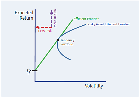
One famous property of the tangency portfolio (or any portfolio on the efficient frontier) is that individual asset expected returns are exactly proportional to beta[6].
E(Ri)-rrisk free=βi[E(RTotal Portfolio) -rrisk free]
If expected returns are not exactly proportional to beta as described above, the investor is not holding the tangency portfolio, and therefore, the investor is not on the efficient frontier. Said another way: If an asset’s expected return is too high relative to its beta, i.e. there is alpha, the portfolio’s Sharpe Ratio could be improved by allocating more to that asset. Thus, statements about alpha are equivalent to statements about whether the investor’s portfolio is on the efficient frontier. A zero (nonzero) alpha implies that the investor’s portfolio is (not) on the efficient frontier. This is why the concept of alpha plays a central role in performance evaluation and portfolio construction. I will return to this important concept in the next section.
Within this MV-MPT framework, it is qualitatively clear how to evaluate new investments. Which new investment increases my total portfolio Sharpe Ratio the most? Equivalently, which new investment improves the efficient frontier the most, i.e. moves it furthest to the left (less risk) and up (more expected return)? In the next section, I will define a simple, easy-to-calculate measure that directly addresses the above, fundamental question.
Before leaving this section, I would like to briefly discuss the above-mentioned model and assumptions. As my dissertation adviser, Eugene Fama[7], used to always say, all models are false by definition. That being said, some models can be a reasonable first-order approximation to the real world, providing valuable insights and reasonable rules of thumb to follow. Additionally, when it comes to learning, I believe in the “first things first” principle – start with the simple model first and move to the more complex only after mastering the simple. If one does not understand/appreciate the implications of the simple model, there is no chance of comprehending the more complex version. For instance, some investment returns exhibit a nontrivial amount of “skewness” and “fat tails” (e.g. short volatility strategies[8]), which won’t be picked up by focusing exclusively on the mean and variance[9]. So, I don’t believe the world of applied portfolio theory is always about mean and variance. However, MV-MPT is a reasonable starting point in addition to providing many valuable, timeless portfolio management lessons.
THE IMPORTANT, YET UNDERUTILIZED, APPRAISAL RATIO
If maximizing the total portfolio’s Sharpe Ratio is the ultimate investor goal under MV-MPT, then the Appraisal Ratio (“AR”) is the relevant risk-adjusted performance statistic when evaluating new investments. In order to clearly define the AR, consider a simple linear regression of the new investment’s excess return (in excess of T-bills) on the existing total portfolio’s excess return.
RexcessNew=α+βRexcessExisting+ε
Alpha, α, is the intercept from the regression while beta, β, is the slope. There is also a regression residual, ε – the part of the new investment’s excess return that can’t be explained by the regression model. The above representation is applicable in both historical and prospective contexts. If historical return information is available, the above regression can be easily estimated. As with any regression, historical relationships only represent what has happened, not what will happen. That being said, if one has a good process for forecasting the inputs (e.g. expected returns, expected volatilities, and expected correlations) to the regression model, it is perfectly valid to utilize the above framework on a prospective basis.
Within this framework, the AR is defined as the alpha, α, divided by the residual volatility, σ(ε).
Appraisal Ratio=α/σ(ε)
Given the “tangency” portfolio results from the last section, it should not be surprising that alpha plays a major role in the AR. When alpha is nonzero, the investor is not on the efficient frontier. In the case of positive alpha, more capital needs to be allocated to the positive alpha asset to improve the portfolio’s efficiency.
Intuitively, why isn’t it enough to just focus on the alpha when evaluating new investments? In order to answer this question, think of the new investment’s return as containing two parts: a unique part and one that is common to the existing portfolio.
The “common” part of the new investment’s return, βRexcessExisting, is irrelevant to improving the efficient frontier. It is already available to the investor via the existing portfolio. On the other hand, the unique part, α+ε, is unrelated to anything available in the existing portfolio and, thus, has potential to improve the efficient frontier. The unique part, however, contains more than just the alpha term. It also includes the unexplained regression residual. This component makes the return’s unique part uncertain or risky, which is undesirable. This is why the AR divides alpha by the residual volatility, σ(ε). Alpha represents the unique part’s expected excess return while the residual volatility represents the unique part’s risk. Based on this representation, I think of the return’s unique part as the realized alpha, where α is the expected alpha and σ(ε) is the alpha volatility. Simply put, the AR becomes a measure of “return per unit risk”, which is similar to a Sharpe Ratio but with a beta adjustment.
While it can be mathematically proven that the maximum attainable total portfolio Sharpe Ratio is directly related to the new investment’s AR, doing so is beyond the scope of this paper.
(Maximum Sharpe Ratio)2=(AR)2+(Existing Sharpe Ratio)2
If we accept the above relationship as true, one can see why the AR is crucial for evaluating investments within MV-MPT. A higher AR translates to a higher Sharpe Ratio for the total portfolio, i.e. a more favorable efficient frontier. This answers the fundamental question addressed in the paper.
At this point, it should be clear why beta-adjusting returns is critical to performance evaluation. In order to calculate the AR, the key performance measure in MV-MPT, returns need to be beta-adjusted[10]. It really is that simple.
In addition to being practical, the AR is easy to calculate. Since the inputs come from widely used linear regression techniques, it can be computed in many software packages, including Microsoft Excel, within seconds. No fancy optimization is needed. Given this, there is no reason to avoid using the AR as one relevant performance evaluation metric.
Although the AR is critical to MV-MPT investment evaluation, it is not well known and, thus, not widely used. To be fair, I only know about it because George Constantinides[11] included it in a problem set for his Asset Pricing Theory course – rather practical for a “theory” class. Clearly, the AR could benefit from a more effective marketing campaign.
A PRACTICAL EXAMPLE
In order to provide better context, the table below reports the AR and various other performance metrics for the following historical example: consider the Swiss Re Cat Bond Index, the Credit Suisse Leveraged Loan Index (Bank Loans), and the MSCI Emerging Markets Equity Index (“EM”) as potential “new” investments, and the “existing” portfolio is allocated to the MSCI World Equity Index and Barclays Global Aggregate Bond Index in a 60/40 split.
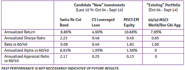
It is interesting to note that EM equities have the highest annualized return but the lowest AR, while catastrophe bonds have a somewhat lower return but the highest AR. Why is this? We know that in the traditional “balanced” 60/40 portfolio, the vast majority of risk comes from the equity component. EM equities are a high-beta form of equity, and therefore most of the risk of an emerging markets equity allocation is common to the existing risk of the 60/40 portfolio. This is why EM equities have a beta of 1.92. In this example, only a small portion, 1.56%, of EM’s annual return is a unique alpha component, and that alpha component is also volatile, producing a low AR.
By contrast, catastrophe bonds have very little risk in common with the 60/40 portfolio, which is consistent with the 0.08 measured beta. Most of the catastrophe bonds’ return is from unique alpha sources (6.91%) with lower volatility, producing a substantially higher AR. As a result, catastrophe bonds are the most impactful addition to the existing 60/40 portfolio.
COMMON PERFORMANCE EVALUATION MISTAKES & MISPERCEPTIONS
As a complement to a paper that advocates the use of the AR, it feels appropriate to address a few of the commonly observed mistakes when it comes to evaluating performance:
- Do not forget to deduct the risk-free rate when estimating alphas.[12] It is common for me to come across analyses – even from vended performance software packages – that forget to work with excess returns. In today’s zero risk-free rate environment, total returns are essentially equal to excess returns, but this has not been the case historically and the deduction of the risk-free rate is a necessary step.
- Unless the investment has zero beta and/or the investor plans to allocate 100% to one investment, do not focus on the individual investment’s Sharpe Ratio. The Sharpe Ratio is a total portfolio performance metric. Unlike the AR, it does not correctly control for the individual investment’s beta.
- Do not be seduced by high average alphas. Similar to total portfolio returns, alphas need risk-adjusting too. The AR is a risk-adjusted measure of alpha.
- Do not necessarily avoid investments with a high correlation to the existing portfolio. A high correlation translates to a low residual volatility, which is a good attribute if the investment has a positive alpha. Remember, the AR is defined as the alpha divided by the residual volatility. A corollary to the above argument: do not necessarily seek investments with a low correlation to your existing portfolio. A low correlation investment with zero alpha is worthless.
- Do not focus too much on individual expected returns. Returns are risky, even over the long run. The expected return represents the “base case” from a distribution with many outcomes below and above. In order to construct a portfolio with the most favorable prospective return distribution, returns need to be appropriately risk-adjusted in the context of the entire portfolio. The AR does just this.
- Lastly, do not forget to beta-adjust returns when evaluating an individual investment’s performance. The AR is a key performance metric, and its components require beta-adjustment.
CONCLUSION
Portfolio construction and performance evaluation are some of the key functions performed by an individual or institution responsible for an investment portfolio. Yet, these important tasks are rarely performed in a manner that is consistent with achieving the highest total portfolio expected return for a given level of total portfolio risk – the investor’s ultimate goal.
Focusing on individual returns does not correct for risk. Focusing on individual Sharpe Ratios does not correct for beta. Focusing on alpha controls for beta but doesn’t account for the alpha’s volatility (risk). Only the Appraisal Ratio, defined as the expected alpha-to-alpha (residual) volatility ratio, correctly accounts for an individual investment’s return attributes. In sum, the new investment with the highest AR delivers the highest total portfolio Sharpe Ratio, i.e. moves the efficient frontier furthest to the North (more expected return) and West (less volatility). This is why the AR is the most relevant performance metric in a MV-MPT world.
ABOUT THE AUTHOR
Mr. Hecht is a Vice President and Senior Investment Strategist at Evanston Capital Management, LLC (“ECM”). Prior to joining ECM, Mr. Hecht served in various portfolio manager and strategy roles for Allstate Corporation’s $35 billion property & casualty insurance portfolio and $4 billion pension plan. He also had the opportunity to chair Allstate’s Investment Strategy Committee, Global Strategy Team, and Performance Measurement Authority. Mr. Hecht also served as an Assistant Professor of Finance at Harvard Business School. His research and publications cover a variety of areas within finance, including behavioral and rational theories of asset pricing, liquidity, capital market efficiency, complex security valuation, credit risk, and asset allocation. Mr. Hecht previously served at investment banks J.P. Morgan and Hambrecht & Quist, and as a consultant for State Street Global Markets. Mr. Hecht has a bachelor’s degree in Economics and Engineering Sciences from Dartmouth College and an MBA and Ph.D. in Finance from the University of Chicago’s Booth School of Business.
EVANSTON CAPITAL MANAGEMENT
Founded in 2002, Evanston Capital Management, LLC is an alternative investment firm with approximately $4.9 billion in assets under management. ECM has extensive experience in hedge fund selection, portfolio construction, operations and risk management. The principals collectively have more than 75 years of hedge fund investing experience, and the firm has had no turnover in senior or mid-level investment professionals since inception. ECM strives to produce superior risk-adjusted returns by constructing relatively concentrated portfolios of carefully selected and monitored hedge fund investments.
The information contained herein is solely for informational purposes and does not constitute an offer to sell or a solicitation of an offer to purchase any securities. This information is not intended to be used, and cannot be used, as investment advice, and all investors should consult their professional advisors before investing in an Evanston Capital Management, LLC (“ECM”) product. The statements made above constitute forward-looking statements. These statements reflect ECM’s subjective views about, among other things, financial products, their performance, and future events, and results may differ, possibly materially, from these statements. These statements are solely for informational purposes, and are subject to change in ECM’s sole discretion without notice to the recipient of this information. ECM is not obligated to update or revise the information presented above.
1.Of course, assumptions are necessary for this result, which will be briefly addressed later in the paper.
2.Variance = volatility squared
3.Sharpe Ratio=(E(R_(Total Portfolio) )-r_(risk free))/σ(R_(Total Portfolio) )
4.Using matrix notation, the tangency portfolio weights are proportional to Σ^(-1) ▁μ^e, which is the inverse of the covariance matrix multiplied by the expected excess return vector.
5.The risky asset efficient frontier excludes the risk-free asset.
6.β_i=Cov(〖R_i,R〗_(Total Portfolio) )/(σ^2 (R_(Total Portfolio) ) )
7.Eugene Fama is a University of Chicago Finance Professor and 2013 Nobel Prize winner.
8.Selling out of the money put options is an example of a short volatility strategy.
9.Jerek and Stafford (“The Cost of Capital for Alternative Investments”, 2013) evaluate hedge funds using a more complex model. Ingersoll, Spiegel, Goetzmann, and Welch (“Portfolio Performance Manipulation and Manipulation-proof Performance Measures”, 2007) discuss the limitations of various “mean-variance” performance measures.
10.Realized Alpha=α+ε=R_New^excess-βR_Existing^excess. The red represents the beta adjustment.
11.George Constantinides is a University of Chicago Finance Professor. Note that Treynor and Black (“How to Use Security Analysis to Improve Portfolio Selection”, 1973) first introduced the Appraisal Ratio concept.
12.Deducting the risk-free rate is not necessary when working with zero-investment, i.e. long/short, portfolios.
RELATED ARTICLES
The Truth About Hedge Fund Risk
A Response from Con Keating to “The Truth About Hedge Fund Risk”
interesting